Interpolation

INTERPOLATION (interpolatio), the supplementing of an empirical series of values of a quantity with missing intermediate values. Interpolation can be performed in three ways: mathematical, graphical, and logical. They are all based on the common hypothesis that the entire series of values of the quantity under study is subject to one general law of distribution and that the value of each member is determined by its position in the series. The degree of reliability of this assumption in each specific case of interpolation determines the degree of approximation of the quantities obtained as a result. 'This is why interpolation should be resorted to only with the greatest caution, firmly keeping in mind that interpolated figures, in terms of reliability and authenticity, cannot in any way be placed on a par with figures obtained from statistical calculation' (Kaufman).

Mathematical methods of I. are diverse in content. Elementary methods are based on the assumption that individual members of the empirical series are members of an arithmetic or geometric progression and that therefore the sought values are the missing members of the corresponding progression. Thus, to determine the population size in the years between adjacent censuses for a given area with population p according to the previous census and p₁ according to the subsequent census, by the arithmetic progression method, one should subtract p from p₁, divide the remainder p by the number of years that have passed between the critical moments of both censuses (n), and take the resulting quotient b = d (the difference of the progression) as the annual increment for constructing the arithmetic progression; under these conditions, the population numbers will be equal to: p, p+d, p+2d, p+3d....., p+d(n-1), where p+d(n-1)=p₁.

When interpolating by geometric progression, under the same initial conditions, the inter-census population numbers will be expressed in the form of the following series: p, pq, pq², pq³......, pq^n-1, where pq^n-1 = p₁, n-1 and q^n-1 = p₁: p or q = n√(p₁: p). Population of Germany (in thousands). = p By arith- By geo- Years metic pro- metric pro- By cen- gression gression sus (d=855.9) (q=1.042) - - - -

More complex mathematical methods of I. are based on the assumption that the interpolated values are located on a straight line or a parabolic curve passing through the observed ordinates. Thus, if it is known that according to census data, the number of persons aged 3-6 years was 4,159,000 people, aged 6-9 years - 3,823,000 people, and aged 9-12 years - 3,602,000 people, then to determine the number of persons in each intermediate one-year age group (3-4 years, 4-5 years, etc.), one can use the equation of a second-order parabola: y=ax²+bx+c, where y is the number of persons of a given age, and x is age.

To find the values of the coefficients of the parabolic equation, various methods can be used (in particular, Newton's, Stirling's, Gauss's interpolation formulas, etc., based on the method of finite differences).

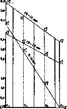
The graphical method of I. consists in finding and measuring on a diagram representing the empirical series those ordinates that correspond to the missing members of the series. For example, to approximately determine the size of three groups of school-age children: 8-9, 10-12 and 13-14 years - as of July 1, 1921, and July 1, 1922, given information about their quantity according to the census of August 28, 1920, and the census of March 15, 1923, one should construct, using millimeter paper, three lines corresponding to the following data of the mentioned censuses (in absolute numbers and as percentages of the total population).

Age According to census According to census of 28/VIII 1920. of 15/III 1923. abs. % abs. % 10-12 years...... 35,279 55,267 36,440 34.3 53.8 35.4 48,322 80,743 51,555 30.0 52.3 33.4

To simplify the construction of the diagram, we will use not the absolute numbers of children, but their percentage content in the total population, and in addition, we will give the abscissa (ox) a variable value: when constructing the ordinates x₁y₁ and x₂y₂, representing the relative number of children aged 8-9 years, we will equate it to 30%, for the ordinates x₃y₃ and x₄y₄, corresponding to the 10-12 year group, we will take it equal to 50% and finally for the ordinates x₅y₅ and x₆y₆ (group 13-14 years) = 30%.

We will plot the initial and sought points of time on the abscissa with such a calculation that each month equals 2 mm. As the initial scale of the ordinates, we will take that every 2 mm of them equals 0.1% (see figure). By tracing the points of intersection of the ordinates corresponding to the sought moments of time with the lines representing the size of the studied children's groups and measuring their distance along the abscissa (ordinates x₂y₁; x₃y₁; x₂y₂; x₃y₂; x₅y₂; x₃y₃), we find that children aged 8-9 years accounted for July 1, 1921 - 32.9% and July 1, 1922 - 31.2%; aged 10-12 years on July 1, 1921 - 53.6% and July 1, 1922 - 52.7%; aged 13-14 years - on July 1, 1921 - 34.3% and July 1, 1922 - 33.9%.

Taking into account that the total number of residents on July 1, 1921 was 1,176.6 thousand people, and on July 1, 1922 - 1,380.7 thousand, we obtain according to the proportions 100:32.9 = 1,176.6:x, 100:31.2 = 1,380.7:x, etc., therefore the number of children (in thousands): age 1921 1922 8-9 years 38.7 40.4 10-12 years 63.1 46.8 13-14 years 48.3 52.3

It should be noted that in the considered example (period 1920 and subsequent years), there were far from ordinary changes in the dynamics of the size of children's groups, which were the result of major demographic shifts in the child population due to a decrease in birth rates during the imperialist war.

The logical method of I. consists in finding, based on certain logical premises, the most probable values of the unknown members of the series. An example of logical interpolation can be the cases of replacing in the temperature curve of certain missing temperature readings in any disease that gives a regular picture of the development of the temperature reaction (typhoid fever, etc.).