Diagram

DIAGRAM, the most common form of graphical representation (see), which consists of using various geometric figures to express certain quantitative properties of phenomena or to express patterns established through statistics. Depending on the nature of the geometric figures, one distinguishes linear, planar, and spatial diagrams. Linear diagrams are those in which the magnitudes of the phenomena under study are expressed by images having one dimension. The most common form of linear diagrams are so-called curves. Their construction utilizes a coordinate system. Coordinates are the values used to determine the position of points, lines, and planes in space. Thus, in Fig. 1 (Table I), the coordinates of point P are the distances PM and PN, or the equal distances ON and OM. The sides of the angle YOX, relative to which the position of point P is determined, are called the coordinate axes, with the side OX being called the axis of abscissas, and OY the axis of ordinates; the angle YOX formed by them is called the coordinate angle. The coordinate ON is called the abscissa, and the coordinate OM is the ordinate. The construction of a curve reduces to the following (Fig. 2, Table I): the axis of abscissas is drawn, and a perpendicular—the axis of ordinates—is erected at its end point; segments corresponding to the adopted units of a given grouping, e.g., individual years (a), are marked off on the axis of abscissas; then, at the end of each such segment—the division of the abscissa—a perpendicular is erected, which is an ordinate parallel to the axis of ordinates (b); further, equal segments proportional to the magnitude of the phenomenon under study, e.g., the coefficient of general mortality, etc., are marked off on the axis of ordinates, and straight lines parallel to the axis of abscissas are drawn from the end points of each segment; this results in a grid (c), on which various expressions of the phenomenon under study (mortality) are marked with points, corresponding to the groupings depicted on the abscissa (years). Finally, the individual points are connected by straight lines, resulting in a broken line (d) or, as it is called, a curve, which gives a clear representation of the gradualness in the changes of the phenomenon being studied. Usually, the measurements of the phenomenon considered to be a factor of the phenomenon under study are plotted on the abscissa. The magnitudes representing the phenomenon considered as a function of the first are plotted on the ordinates; "the result is an image representing different values of the function in direct connection with different values of the producing factor" (Kaufman). This also defines the significance of linear diagrams in the form of curves: in cases where only one curve is plotted on the grid, the purpose of the diagram is to reveal or visually depict the dependence between the factor depicted on the divisions of the abscissa and the function whose values are plotted on the ordinates. Diagrams on which there are several curves sometimes, just like diagrams with one curve, aim to show the dependence of several functional values depicted on the ordinates on the factor depicted on the abscissa. But usually, diagrams with several curves have not so much this goal, but rather the clarification of the interrelation between different functional values that have found expression in different curves, revealing parallelism or antagonism between them. Thus, in the diagram depicted in Vol. IV, art. 211, the intention is not so much to show the change in typhoid fever morbidity and the change in vaccination over a number of years, but mainly to reveal the influence of vaccination on typhoid fever morbidity; likewise, for example, in the diagram depicted in Vol. VIII, art. 45, the intention is not so much to show the change in mortality, birth rate, and typhus morbidity or the change in industrial production, transport work, and the number of workers over a number of years, but rather to reveal the parallelism between the first group of curves, which characterize social health, and the second group of curves, characterizing economic conditions, which are factors of social health. The time segments depicted on the abscissa in this case are simply grouping units. When constructing linear diagrams in the form of curves, the following basic rules must be observed (Janson). 1. The parts plotted on the abscissa must necessarily be equal and correspond to equal magnitudes of the phenomenon depicted on the abscissa. Violation of the latter rule, permitted for example in Fig. 4a, Table I, where in the left half of the diagram each segment of the abscissa corresponds to a period of 10 years, and in the right half of the diagram to a period of 1 year, leads to an incorrect representation of a steeper and sharper decline in infant mortality during the 19th century compared to the 20th century. The techniques applied in Fig. 4b—separating the left half of the diagram from the right with a break in the curve, as well as depicting the left half of the curve with a dashed line, in contrast to the solid line in its right half—can only partially compensate for the violation of the correctness and clarity of the diagram that occurred as a result of allowing different scales in different parts of this diagram. 2. The data or factors must represent a continuous sequential series. A violation of the continuity of this series, for example in the case of missing data for certain years, must be shown by a break in the curve, as is done, for example, in Diagram 10 in Vol. IV, art. 178. 3. The ordinates must depict the full quantities of the phenomenon under study, and not only that part of it which changes, which could give a completely false idea of the degree of variability and fluctuation of the given phenomenon. (For example, Fig. 3, Table I—an incorrect construction of the same diagram that is depicted in Fig. 2: on the axis of ordinates, the divisions start not from 0, but from 14, as a result of which a curve is obtained that gives an idea of sharper relative fluctuations in mortality than actually took place.) 4. The scale or magnitude of the ordinates must show the change in data in an arithmetic progression, and not in a geometric one, with all divisions of the scale being identical: "only a scale constructed in a simple arithmetic progression satisfies the postulate of graphical representations that the curve should connect the ends of lines proportional to the depicted magnitudes" (Mauger). Sometimes, however, statistics use so-called logarithmic scales, in which the segments of the scale are proportional to the logarithms of the numbers, corresponding to the change of logarithms in an arithmetic progression. Meanwhile, as is known, the increase of logarithms in an arithmetic progression corresponds to the increase of numbers in a geometric progression. Therefore, on any logarithmic scale (for example, Fig. 5b, Table I), the distance from 10 to 20 will be the same as from 20 to 40, as from 40 to 80, from 80 to 160, etc. For this same reason, when graphically representing on a logarithmic grid (or rather, a semi-logarithmic one, since usually in these cases an ordinary horizontal and a logarithmic vertical scale are used), any numerical series increasing in a geometric progression forms a straight line, and an identical slope of the curve corresponds to an identical coefficient of increase or decrease, whereas on an ordinary grid, an identical slope means an increase by the same number. Due to the peculiarity of the non-uniform logarithmic scale, diagrams constructed on it are not easily grasped, as a result of which they are used almost exclusively for research purposes when it comes to depicting the expression of growth or decline coefficients, since the relative increase of numbers is reflected on the logarithms of these numbers in the form of an increase by specific terms, which are equal given the same relative increase of numbers. Thus, in Fig. 5a and b, Table I, an image of the same phenomenon is given on an ordinary and a logarithmic grid: the number of inhabitants over a number of years in a city with an initial population of 10,000 people with a growth of 20% every 10 years (as a result of the same relative growth, a straight line is obtained on the logarithmic grid). The logarithmic grid further makes it possible to place on one drawing the results of observations whose numerical values are so far apart that depicting them on one drawing with ordinary scales would force the use of too small a scale, at which the difference between small numbers would be barely noticeable. Meanwhile, on a logarithmic scale, small numbers are represented by relatively larger divisions than large numbers, and the upper part of the diagram is, as it were, in a condensed form (Fig. 5b). 5. A large number of curves can be plotted only if the scale of the diagram is sufficiently large; otherwise, the intersection of a large number of lines will not allow one to follow the course of each line and the interrelation of the fluctuations of different lines. 6. When choosing a scale for the axis of abscissas and ordinates, one should strive to ensure that the character of the resulting curve (i.e., the degree of its jaggedness or, conversely, its flatness) corresponds to the degree of actual constancy or variability of the phenomenon.

Thus, the use of different scales for the scales on the abscissae and ordinates in Fig. 6 a and b when constructing diagrams illustrating one and the same phenomenon (the decline in mortality in German cities over a number of years) leads to completely different ideas about the nature of the phenomenon being studied (mortality): figure 6a creates the impression of a sharp decline in mortality; in Fig. 6 b, due to the fact that the scale on the ordinate axis is smaller and the scale on the abscissa axis is larger than in Fig. 6 a, the impression of a slower decline in mortality (a flatter curve) is obtained. Linear diagrams in the form of curves are used a) to express changes in various phenomena over time (see, for example, diagrams in Vol. IV, pp. 670, 672, etc.); b) to depict the dependence of various phenomena on certain factors that are amenable to uniform, continuous quantitative gradation, for example, to depict changes in morbidity, mortality, nutrition, etc., depending on the size of income; to depict age-related changes in height, weight, marriage rate, mortality, etc. In these cases, the curve best reveals the trend of change in a given phenomenon depending on factors arranged in a certain gradation; c) to depict the various quantitative distributions of some trait in a given aggregate, the so-called "distribution curve" in variational statistics (figure in Vol. IV, p. 422). Linear diagrams also include diagrams on a system of so-called polar coordinates (radial diagrams), in which various magnitudes of phenomena are depicted by different segments of the radii of a circle. Diagrams of this type are used in cases where it is intended to depict phenomena that close and renew themselves in a known cycle, exhibiting regular periodicity, for example, the distribution by months of the year of marriages, births, deaths, or the distribution by days of the week of accidents, etc. Usually, the radius of the circle is taken to be equal to the average of the monthly or weekly figures; in such a case, it will be clear at a first glance which months or days yield figures above or below the average (Table I, figure 7). In this case, the radii corresponding to different months of the year or different days of the week are plotted in a clockwise direction, starting from the position corresponding to the position of the clock hand at 12 o'clock (January in Fig. 7). Some statisticians deny the expediency of polar diagrams (Schwabe); others point to graphic optical illusions when they are perceived by viewers (Whipple); however, one should agree with Kaufmann that only on a polar diagram will adjacent months in time, December and January, be depicted adjacently, and yet these months are very close to each other both in climatic and in some economic conditions; it is precisely on a polar diagram that the influence of Sunday revelry on the increase in the number of accidents, which also extends to the following two days of the week (hangover), and often even to Saturday (payday), is best revealed.

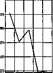
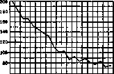
Planar (planimetric) diagrams are called those diagrams in which geometric figures having two dimensions (rectangles, squares, triangles, circles, etc.) are used. In this case, the figures are drawn to such a scale that the ratios of their areas correspond to the ratios of the magnitudes they depict. Therefore, when using the form of squares or circles, the sides of the squares or the radii of the circles must be calculated by extracting the square root of the ratio between the magnitudes; when using rectangles with equal bases (bar diagram), the ratio between the magnitudes is equal to the ratio of the heights of the rectangles, etc. (Fig. 1, Table II). In statistics, two types of planar diagrams are used: separate, or isolated, and connected. Isolated diagrams are used: a) for comparing magnitudes independent of each other (unlike linear diagrams, where the depicted phenomena are considered as functions of other phenomena), for example, population size or birth rate and morbidity in different countries, provinces, etc. (see Diagram 9, Vol. IV, pp. 178-179, "Morbidity from typhoid fever in different states in 1926" and "Morbidity from typhoid fever in individual provinces of the RSFSR", or Diagram 1, Vol. IV, pp. 637-638, "Spread of syphilis by individual provinces"); b) for depicting the breakdown of a mass into its constituent parts, i.e., for depicting coefficients of extensivity. Rectangles and circles are most often used for the latter purpose. In a rectangle, the ratios of the magnitudes are equated to the ratios of the segments of the height (Fig. 2 A, 2B, Table II). In a circle, the whole is taken as equal to 360°, and for each component, a sector of the corresponding number of degrees is determined (1% equals 3.6°) - a sector diagram (Fig. 2B, 2G, Table II). Connected, or complex, planar diagrams, like linear ones, are built on a straight line taken as the abscissa, on which equal parts are plotted. The magnitudes subject to construction are divided into two factors, of which one, common to all, is a part of the abscissa. From this, it is clear that the figures built on the abscissa can only be either rectangles or triangles. Preference should be given to the former in this case, since it is more convenient to plot the constituent parts of the whole on them, i.e., the internal breakdown of one or another phenomenon. Planar connected diagrams are used a) for depicting the change of some phenomenon both as a whole and in its breakdown into constituent parts, for example, the gradual growth of a revenue or expenditure budget with its distribution by items (Fig. 2 and 3, Table II), b) for depicting the parallel change of several series of phenomena independent of each other. The demonstrative value of complex planar diagrams is beyond doubt. However, in terms of analytical value, planar diagrams are far inferior to a simple linear diagram, since on a planar diagram, one can never plot as many phenomena as on a linear one. But a planar diagram also has an advantage: only it allows depicting Table I. b. 1912 \ \ \ Figure 1. Coordinate system. Figure 2. General mortality in the city of Moscow 1920-1924. The beginning of the divisions on the ordinate is not from zero", "1920|1921|1922|1923|1924 Figure 3. The same material as in Fig. 2 when constructing a diagram on ordinary (a) and logarithmic (b) scales. 6o--The curve gives a distorted idea of the rate of decline in infant mortality in the 19th and 20th centuries 200 ' ' 180- \ \ \ ', ^ * ^ Ch,- Weakening of the shortcomings of diagram 4d. by a break in the curve and its different depiction (dashed and solid line) | 901 B 1L E 1 321 (831 [ asyuk so vy t 8JI yus X» 10! 9M 9Ya 1P *Ya Id No Kb Figure A. Infant mortality in the 1st year of life per 1000 born in Sweden. CHOICE OF SCALE WHEN CONSTRUCTING A CURVE. (a) / y s 1870 1880 1890 1900 1910 \\b\\ > I' / Fig. 5. Number of inhabitants in city A from 1870 to 1930. || 1 " sh ' go» G(T1 1UU »i lljlll II 1 1.1. II . and 780 86 90 fi Ya OM os sh sh Curves in Fig 6a..and 6b constructed on the basis of the same data give a different idea of the rate of decline in mortality, due to the use of different scales during construction. POLAR COORDINATES. The curve in Fig. 6b..due to the proportional reduction of the scale, retains the same character as in Fig. 6a. * -i g 180 : 7 80 85 90 109 »(5 Figure 6. Mortality of the population in German cities per 1000 inhabitants from 1877 to 1905."

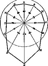
Fig. 7. Infant mortality by months of the year in European Russia at the age from 0 to 1 year.

Table II.

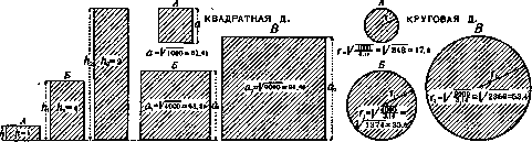
Fig. 1. Population size in different cities: A-1000 people. B-4000 people. C-9000 people. DEPICTION OF THE BREAKDOWN OF A MASS INTO ITS CONSTITUENT PARTS.