Variational Statistics

VARIATIONAL STATISTICS, a term uniting a group of statistical analysis methods used predominantly in the natural sciences. In the second half of the 19th century, Quetelet (Quetelet, "Anthropometrie ou mesure des differentes facultes de l'homme", 1871), and then Galton (Galton, "Natural inheritance", 1889) used statistical research methods to solve natural science problems; by the end of the 19th century, the application of the statistical method in natural science had already become widespread. This necessitated the refinement of old and the creation of new methods of statistical analysis in connection with the peculiarities of research material in natural science. The term "mathematical statistics" appeared to designate that branch of statistics in which the methods and techniques of mathematical analysis, predominantly probability theory, are widely used. Alongside this, on the threshold of the 20th century, the term variational statistics also became widespread, emphasizing by its name the predominance of variability issues in those areas where the statistical methods united by this term are applied. The word "variational" is usually derived from variation, variant, and varying (i.e., change, changing object, the fact of variability). It is impossible to draw a strict demarcation between mathematical statistics and variational statistics: both treat the same research methods and consider the same techniques. The term variational statistics spread predominantly in Central Europe and from there penetrated to us. However, its founder is justly considered to be the English scientist K. Pearson, who published, starting in 1894 ("Contribution to the mathematical theory of evolution"), many works concerning the theoretical substantiation of statistical research methods as applied to natural science issues (see also Biometry). Over the last 25 years, variational statistics has been developing rapidly, and its methods are applied in the most diverse fields of knowledge; in medicine, the application of variational statistics has become widespread predominantly in anthropometry, physiometry, and psychometry, and in the doctrine of constitutions. At present, variational statistics is taught in medical faculties under the department of social hygiene; on the biological divisions of the physics and mathematics faculties, a special course in biometrics and variational statistics has been introduced, and in the mathematical divisions, there is a special branch of mathematical statistics. Variational statistics is used in many research institutions (Institute of Social Hygiene, anthropological institutes, etc.), is widely used in pedology; many issues in special medical works dealing with mass variable material are solved using variational statistics, so that for the physician variational statistics is becoming one of the working tools. The explanation for the development of variational statistics in recent years and its wide penetration into various sciences must be sought 1) in the need to systematize the abundant research material accumulated in recent years, 2) in the refinement of the methods (techniques) of scientific work, and 3) in the general tendency of scientific thought to replace qualitative formulations with quantitative expressions. The study of a mass phenomenon is conducted in the form of investigating a statistical aggregate, which is the main subject of statistics. Variational statistics deals predominantly with the study of the statistical aggregate in terms of quantitatively varying attributes, and gives some general guidelines on evaluating the results of research. Attributes subjected to statistical analysis can be qualitative (gender, color, disease, etc.) or quantitative (weight, dimensions, % hemoglobin, etc.), and the study of the statistical aggregate can be conducted either for each attribute separately or simultaneously for two, three, or more attributes; in the latter case, the question of mutual correspondence and mutual dependence of attributes arises, and the question of correlation is posed (see). The study of an aggregate by a single attribute, in the case of its qualitative character, is often limited to a simple indication of the proportion of a given category of attribute in the surveyed aggregate (% of men, % of lymphocytes in the blood); in the case of a quantitative attribute, summary characteristics of the entire aggregate are given, i.e., certain numbers are determined that summarily characterize this aggregate according to the studied attribute (% of objects with a certain category of qualitative attribute can also be considered a summary characteristic of the aggregate). The statistical aggregate to be studied can be given in two forms: 1. The values of the attribute are directly indicated for all objects of the aggregate: where the various x are the varying values of the attribute, and N is the total number of objects in the aggregate, called the volume of the aggregate. Volume is the main characteristic of the investigated aggregate. Example: x = % of lymphocytes in Moscow schoolgirls aged 9 years to 9 years 11 months (according to the materials of the Office of School Pedology of the Academy of Communist Education, work of Dr. Chetunov); x: 23 25 26 27 27 28 28 30 30 30 31 32 32 33 35 37 38 40;

Thus, an aggregate of small volume (N not greater than 40-50) can be given. 2. An aggregate of larger volume is given in the form of a double series: a) of attribute values and b) of numbers of observations corresponding to each value, called frequencies x₁, x₂, x₃, ..., x_n, and n₁, n₂, n₃, ..., n_n (II), where x_i are the values of the attribute, and n_i are the corresponding frequencies. It is obvious that n₁ + n₂ + n₃ + ... + n_n = N; more briefly this can be written as Σn_i = N. *(1) The values of the attribute in the second case are usually given in the form of intervals, otherwise called class intervals. Example: x = birth weight, excluding premature and macerated infants, in kg. x: 1.5 - 2 - 2.5 - 3 - 3.5 - 4 - 4.5 - 5 - 5.5 n: ... (IIa). Series similar to series (I) and (II) are called variational series. The question of the magnitude of the interval for the variational series (II) is solved depending on the characteristics of the investigated material. One can only recommend conducting primary observations (measurements) in the smallest possible intervals, then, during tabulation (depicting the obtained observations in the form of a table, in the form of a variational series), reducing them (forming larger intervals from small ones). Successful reduction facilitates the study of the aggregate, keeping in mind that too small intervals complicate the study of the statistical aggregate (calculations and establishment of regularities in the change of frequencies when attribute values change), and too large intervals coarsen the research material. For greater clarity and more detailed study, variational series similar to series (II) are depicted graphically a) either in the form of a series of rectangles with heights proportional to the frequencies (histogram according to Pearson, see figure 1), b) either in the form of a polygon (frequency distribution polygon),

Figure 1. Histogram. obtained after connecting with straight lines the upper ends of the perpendiculars proportional to the frequencies and erected from the midpoints of the corresponding intervals (see figure 2**). In cases where the broken line of the variational polygon is replaced by a smooth curve, the latter is called a variational curve or distribution curve. The first step in the study of a statistical aggregate is the establishment of a summary characteristic of the typical, generally average, value of the attribute in the aggregate. The average value is constructed differently depending on the properties attributed to it.

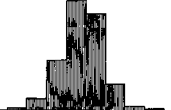
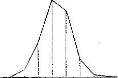
1500 - 2000 - 2500 - 3000 - 3500 - 4000 - 4500 - 5000 - 5500 Figure 2. Polygon. 1. If we consider as typical and characteristic that which occurs most frequently, we must adopt the "mode" (der dichteste Wert, designation: Mo) as the average—the value of the character that has the highest frequency [with such a roughly approximated value of the mode for example (IIa) being the midpoint of the interval from 3,000 to 3,500, i.e., Mo = 3,250 g]. With this elementary construction of the average, the values of the character in objects not belonging to the modal group are not taken into account. For a variational series with a small N [example (Ia)], it is difficult to establish the mode; sometimes the mode can be revealed by repeated grouping, changing the interval boundaries. The exact calculation of the mode is associated with determining the equation of the theoretical distribution curve corresponding to the given variational series. Geometric definition: the mode is the abscissa of the highest ordinate of the variational curve. The calculation of the mode can be somewhat refined if we take into account the frequencies of the two intervals adjacent to the modal one. E. Czuber proposes the following approximate formula for the mode: Mo' = x_i-1 + Δ * (n_i - n_i-1) / (2n_i - n_i-1 - n_i+1), where x_i-1 denotes the lower boundary (in the direction of smaller values) of the modal interval, Δ is the magnitude of the interval, and n_i-1, n_i, and n_i+1 are, respectively, the frequencies of the intervals: the one preceding the modal, the modal one, and the one following it. For example (IIa) Mo' = 3,000 + 500 * (487 - 254) / (2 * 487 - 254 - 311) = 3,414 g.

2. If we consider characteristic and typical for a given population that which is furthest removed from the extreme (atypical) values, we must adopt as the characteristic of the "average" the value of the character in the middle, central object in a ranked population (objects are arranged in order of increasing or decreasing values of the character), called the "median" (der Zentralwert, designation: Me). Me divides the population into two equal halves: the lower one, with values less than Me, and the upper one, with values greater than Me. As a summary characteristic, Me is most frequently used in the processing of test results. The determination of Me for a population with a small N reduces to directly indicating the value of dCh-1

, of the character for the (N + 1) / 2-th object in the ranked population when N is odd; when N is even, the average between the values of the character for the N / 2-th object and the (N / 2 + 1)-th object is taken [in example (Ia) Me = 30]. In the case of populations with a large N, for the elementary calculation of Me from the series of frequencies, a series of cumulative sums is compiled (the frequency of the first interval is added to the frequency of the second, the frequency of the third to the obtained sum, etc.; denoting the cumulative sums by S, we have: S₁ = n₁; S₂ = S₁ + n₂; S₃ = S₂ + n₃ = n₁ + n₂ + n₃, etc.) and, comparing the cumulative sums with N / 2, we determine in which of the intervals Me lies; to its lower boundary is added a part of the interval equal to the ratio of the difference between N / 2 and the cumulative sum of the previous interval to the frequency of the median interval: Me = x_i-1 + Δ * (N / 2 - S_i-1) / n_i, where x_i-1 is the lower boundary of the interval in which the median lies, Δ is the magnitude of the interval, S_i-1 is the cumulative sum of the previous interval, and n_i is the frequency of the median interval. For example (IIa) x: 1.5 - 2 - 2.5 - 3 - 3.5 - 4 - 4.5 - 5 - 5.5 kg n:

5 53 254 558 487 127 19 2 S: 5 58 312 870 1357 1484 1503 1505 ~- 752.5; D = 500; 2 ' Me = 3.000 + 500-^Ь^³-== 3.396g. With such a calculation of Me, it is assumed that within the median interval the values of the character are distributed evenly. More precise calculations of Me, as well as Mo, are associated with the determination of the theoretical variational curve. Geometric definition: Me is the abscissa of that ordinate of the variational curve which divides the area of the curve in half. Me, taking into account the values of the character in objects in the order of their sequence, does not take into account the magnitudes of the values of the character: one can vary the values of the character in the lower half in any way, as long as they do not exceed Me, and in any way in the upper, as long as all are greater than Me; to such variations Me will be insensitive, it will remain unchanged. 3. The simplest and most recognized summary characteristic of the "average" value, which also takes into account the actual values of the character, is the arithmetic mean M (das arithmetische Mittel), defined by the formula: X₁+X₂+X₃+...+X_N M = (1), M~ (2). which is more briefly written: 2x If each value of the character corresponds to a certain frequency (n), then "Znx dr = (3), i.e., the sum of the products of each x by the corresponding n, divided by N. M indicates that value of the character which would be in all objects if the values of the character were distributed equally among all objects (average wage, average height, etc.). If the value of at least one of the objects changes, then M will also change, 1 true, by only the js-th of the change in the character of an individual object. In addition to the indicated means Mo, Me, and M, in variational statistics, the geometric mean M_g and the harmonic mean M_h are sometimes (comparatively rarely) used. The geometric mean of N any quantities is called the N-th root of the product of these quantities Mg = ^N√x₁.x₂.x₃...x_N and is calculated by the formula: log M_g = ~ s log x_{; the harmonic mean of N numbers is the quantity inverse to the arithmetic mean of the inverse values of these numbers: M_h = _{t t} In special ~y2-1~~x cases, summary characteristics of the average and other constructions are possible. With the help of one or another mean, the characteristic value of the character in a given population is revealed; however, one such summary characteristic is not enough: for two populations, with different values of the character in objects, the means can be the same (9, 10, 11, 12, 13, 14, 15—their M = Me = 12 and 3, 5, 9, 12, 15, 18, 22—also M = Me = 12). This difference in general form is expressed by the difference in the dispersion of the values of the character. Greater or lesser dispersion to a certain extent determines the reliability, significance of the mean as a characteristic value: the more dispersed the values, the less reliable the "average". Therefore, usually together with the average value, a summary characteristic of dispersion is also indicated; this is the second step in the study of a statistical population. 1. The most elementary way to determine dispersion is to indicate the limits of variation, maximum and minimum values of the character (sometimes the amplitude, the difference between maximum and minimum, is used). However, this cannot be considered a summary characteristic of dispersion, since maximum and minimum determine only two extreme values, which are the least characteristic of the entire population as a whole. Maximum and minimum are used only in cases where it is especially important to know the limits of variation of the character. 2. As other indicators of dispersion, by analogy with Me, the values of the character in the middle objects in the lower and upper halves of the population, cut by Me, are taken. The lower (first) quartile (Q₁)—such a value of the character, less than which has the values of the character of ¹/₄ of all objects, and, consequently, greater than which—³/₄ of all objects; the upper (third) quartile (Q₃)—such a value of the character, less than which have the values of the character of ³/₄ of all objects, and, consequently, greater than—¹/₄ (it is obvious that Q₂=Me). Having indicated Q₁ and Q₃, the limits of variation of the character in the central (inner) half of the population are determined thereby. Sometimes the following quantities are used as measures of dispersion: q₁=Me-Q₁, q'=Q₃-Me and g_n = q₁+q' Q₃-Q₁ which can be called the lower, upper, and middle quartile deviations (in the terminology concerning quartiles, there is no unity; in some German manuals, q₁ and q' are called the lower and upper quartiles; this article indicates the original, more widespread English terminology). In some cases, deciles and even percentiles are also used. The first decile is such a value of the character, less than which has the value of the character of 1/10 of all objects; percentiles are the same about hundredths of all objects. Quartiles are calculated in the same way as the median; only ¹/₄ N should be replaced by ¹/₄ N for Q₁ and ³/₄ N for Q₃. Quartiles, just like Me, do not take into account the actual magnitudes of the values of the character, dealing only with their ordered sequence.

To take into account the actual magnitudes of the values of the character, sometimes as a measure of dispersion the arithmetic mean of absolute (disregarding the sign + or -) deviations from the mean is used, called the average deviation (die durchschnittliche Abweichung), # = -*- [straight lines indicate that only absolute values of differences (x-M) are summed]. For any series of numbers (x) one can indicate another value, different from M, the arithmetic mean of absolute deviations from which is also equal to #; therefore, formula # ' = -^f-K is sometimes used, since Me for any series of numbers will be the single value, smallest in relation to absolute deviations from it. from the arithmetic mean of the squares of deviations from M. Designation and formula a=m/ ^£<x-M>? (4a), or, if frequencies are given, (in relation to a, the arithmetic value is the single one, since the sum of the squares of deviations from M for any series of values is less than the sum of the squares of deviations from any other value different from M). Through s, the question of the limits of the typical and normal is solved. Measures of dispersion are also absolute measures of variability of the character, expressed in the same units (kg, cm, etc.) as the values of the character. Often the study of a statistical population by a single character is limited to the determination of the average characteristic and the corresponding measure of dispersion. 5. If it is necessary to compare the variability (dispersion) of two different characters, then from M and a a relative measure of variability is obtained, the coefficient of variation, defined as the ratio of a to M expressed in %: m 100% (5). [Similarly for the median and the semi-interquartile deviation 2M 100%, the latter value in cases close to normal distribution (see below) is 1 1/2 times smaller than V]. The calculations of M and a both for large populations and for populations with a small N are best carried out using an arbitrary mean (A). Some number (any number, for convenience of calculation better closer to the average values) is taken as A, then with a small N the entire series of x's is rewritten as a series of deviations from A, a series of a's is obtained, each a = x - A; the last series is summed, and the correction is determined: v = -^-; the arithmetic mean is determined by the formula: M = A + v, "(6), to calculate a, a series of a²—squares of deviations from A—is compiled, and the formula is used:

_______ (7)- UT^> For example (1a), the record of calculations M я and + 1 + 2 + 2 + 3 + 5 + 7 + 8 40 + 10 100 N = 18; A = 30; S₀ = + 12; v = + 0.67; M = 30 + ( + 0.67) = 30.67% lymph.; S₀' = 372; = 20.6667; -»= 0.4444; s = l/20.6667 - 0.4444 = 4.50% lymph. 4. However, the most widespread and recognized measure of dispersion, which also takes into account the actual magnitudes of the values, is the standard deviation, otherwise called the root-mean-square deviation, defined as the square root In the case of a large N, when the population is distributed by intervals, frequencies are adjusted to the midpoints of the intervals ("weighted ordinates method", according to Pearson), and the calculations of M and s are also carried out using an arbitrary mean; the midpoint of some interval is taken as the arbitrary mean (A), and a refers to deviations from the arbitrary mean, expressed in numbers of intervals (deviation of one interval, deviation of two intervals, etc.). Having designated the magnitude of the interval D as before, for the calculation of M and s such formulas are obtained: M = A + v · i, where <=-^'^X"]

(9). The calculations are arranged as follows (example IIa): x (in kg) n a pa pa² 1.5–2.0 -3 -15 2.0–2.5 -2 -106 2.5–3.0 -1 -254 3.0–3.5 0 0 3.5–4.0 + 1 + 487 4.0–4.5 + 2 + 254 4.5–5.0 + 3 + 57 5.0–5.5 + 4 + 8 N = 1,505; Σpa = + 431; Σpa² = 1,709; A = 3.250; i = 500; v = + 0.287; M = 3.250 + (+ 0.287) × 500 = 3,394 g; σ² = 1.1355; σ = 1.0656; σ = 1.0656 × 500 = 532.8 g; σ₁² = 1.1355 - v² = 1.1355 - 0.0825 = 1.0530; σ₁ = 500 × √1.0530 = 513 g. In addition to the indicated simple summary characteristics (mean and dispersion), when studying a variational series (type IIa), higher-level summary characteristics are sometimes used, associated with the problem of the frequency distribution of a given population according to the corresponding values of the attribute. In relation to the distribution, dispersion is a particular property; in addition to dispersion, the asymmetry of the distribution and its greater or lesser flattening or peakedness are studied. Further deepening of the study of a population distributed according to a single attribute is achieved by a more complex mathematical analysis of the distribution, based predominantly on probability theory. Methods for studying a population distributed according to two, three, or more attributes constitute the subject of correlation theory (see), which is also one of the branches of variational statistics. The results of the study of statistical populations are compared with each other, and through this comparison, certain conclusions are outlined and determined. Skillful and correct comparison of the study results is a matter not only of statistical technique and, in a certain sense, statistical art, but also to a large extent depends on the researcher's orientation in the field of the phenomena being studied and the completeness of information about the material being studied. Using the study results in conclusions, one should remember that statistical numbers differ in their nature from arithmetic numbers; statistical numbers do not possess that absolute significance (reliability) which is inherent in numbers in arithmetic; statistical numbers are almost all associated with a greater or lesser probability, which ultimately is determined by the conclusion being made. Along with summary characteristics, their standard errors are usually indicated, determined by the formulas: standard error of the arithmetic mean s_M = σ/√N; standard error of the standard deviation s_σ = σ / √(2N); probable errors are sometimes applied P_M = 0.67449 (× σ/√N), P_σ = 0.67449 (× σ / √(2N)). Probable errors for the median and quartiles P_Me = 0.8454 (× σ/√N), P_Q = 0.9191 (× σ/√N). Mean and probable errors are usually appended with a sign (+, -) to the corresponding characteristics and show the limits of possible variations of the characteristic: standard errors within 0.67449 (about ²/₃) of all theoretically admissible variations for a given characteristic, probable errors within 0.5 of all variations. For example (IIa): e_M = 513 / √1505 = 13.2 g; s_σ = 513 / √3010 = 9.36 g, i.e., the arithmetic mean of the weight of newborns under the conditions of old St. Petersburg lies, approximately (two chances against one), within the limits of 3380.2–3407.2 g, and the standard deviation within 503.4–522.6 g. Standard and probable errors first of all make it possible to compare the relative significance of the same characteristics of several populations, and can also be used to evaluate the results of comparisons; e.g., to establish the reliability of the difference between two statistical characteristics, a triple standard error (+3e) or 4¹/₂ probable errors (+4¹/₂P) is sometimes used. Standard and probable errors were initially introduced for the Gaussian law of random errors, and only later became widespread as estimates of summary characteristics of a statistical population; therefore, their application is associated with the admission in one form or another of an element of randomness in the obtained characteristics, and in the absence of it, errors appear only as if new expressions of dispersion. The concrete interpretation of errors, associated with theoretically admissible variations of summary characteristics, is largely determined by the peculiarity of the phenomenon being studied and the features of the material subjected to statistical processing. In a more general form, errors, like many other results of statistical processing, are associated with certain problems of probability theory. In general, embarking on the path of statistical processing, the researcher will constantly deal with probabilistic judgments, and his advantage over a person not using the statistical method will also lie in knowing the magnitude of the probability of his judgments, not counting the main purpose of the applications of the statistical method—to perceive in the mass such quantitative details of the studied phenomenon that are inaccessible to observation in individual cases.